前言
caffe是个很好用的机器学习工具,尤其是在图像处理做卷积神经网络方面。要掌握caffe,最主要的要掌握:
- 数据生成
- 网络结构定义
- solver配置文件参数设置
接下来我逐一为大家介绍。
生成LMDB数据
数据下载
这次项目是实现500张5个类别.jpg图片的训练和测试识别。在这里为大家提供了数据源的链接:https://pan.baidu.com/s/1MotUe
这些数据共有500张图片,分为大巴车、恐龙、大象、鲜花和马五个类,每个类100张。编号分别以0,1,2,3,4开头,各为一类。
生成图片清单文件
创建一个sh脚本文件,调用linux命令生成图片清单(当然你喜欢的话,你也可以自己写):sudo vi examples/images/create_filelist.sh
在这个文件中输入如下代码并保存
|
|
运行
sudo sh examples/images/create_filelist.sh
类似的生成相应的测试图片清单(其中相关了命令不在此介绍,可自行百度)。
最终生成train.txt文件如下(test.txt类似):
|
|
生成lmdb数据文件
由于参数较多,我们还是创建sh脚本文件运行(这样也比较酷):sudo vi examples/images/create_lmdb.sh
编辑并保存:
|
|
其中设置参数shuffle打乱图片顺序,为了快速学习,将图片大小resize成38*38(硬件受限,这样程序跑的快一点)。然后输入sudo sh examples/images/create_lmdb.sh
运行程序,生成所要的数据文件。
生成图片均值文件
为了提高速度和精度,我们一般还会计算并让图片减去均值,这个用caffe自带的工具函数就能实现:
|
|
第一个参数:examples/mnist/mnist_train_lmdb, 表示需要计算均值的数据,格式为lmdb的训练数据。
第二个参数:examples/mnist/mean.binaryproto, 计算出来的结果保存文件。
网络层layer介绍
这个部分我们就简绍卷积神经网络中最主要的两个层卷积(convolution)层和池化(pooling)层。
Convolution层
就是卷积层,是卷积神经网络(CNN)的核心层。
示例如下:
|
|
主要参数介绍:
num_output: 卷积核(filter)的个数
kernel_size: 卷积核的大小。如果卷积核的长和宽不等,需要用kernel_h和kernel_w分别设定
其它参数:
stride: 卷积核的步长,默认为1。也可以用stride_h和stride_w来设置。
pad: 扩充边缘,默认为0,不扩充。 扩充的时候是左右、上下对称的,比如卷积核的大小为5*5,那么pad设置为2,则四个边缘都扩充2个像素,即宽度和高度都扩充了4个像素,这样卷积运算之后的特征图就不会变小。也可以通过pad_h和pad_w来分别设定。
weight_filler: 权值初始化。 默认为“constant”,值全为0,很多时候我们用”xavier”算法来进行初始化,也可以设置为”gaussian”
bias_filler: 偏置项的初始化。一般设置为”constant”,值全为0。
bias_term: 是否开启偏置项,默认为true, 开启
group: 分组,默认为1组。如果大于1,我们限制卷积的连接操作在一个子集内。如果我们根据图像的通道来分组,那么第i个输出分组只能与第i个输入分组进行连接。
Pooling层
也叫池化层,为了减少运算量和数据维度而设置的一种层。
示例代码:
|
|
主要参数介绍:
- kernel_size: 池化的核大小。也可以用kernel_h和kernel_w分别设定。
其它参数:
pool: 池化方法,默认为MAX。目前可用的方法有MAX, AVE, 或STOCHASTIC
pad: 和卷积层的pad的一样,进行边缘扩充。默认为0
stride: 池化的步长,默认为1。一般我们设置为2,即不重叠。也可以用stride_h和stride_w来设置。
pooling层的运算方法基本是和卷积层是一样的。
我的网络模型
包括一个数据层,两个卷积层,两个池化层和两个全连接层。
|
|
solver文件介绍
solver文件可以算是caffe里最核心的文件了,它就相当于是电脑的CPU,控制着整个网络的运行。
在每一次的迭代过程中,solver做了这几步工作:
- 1、调用forward算法来计算最终的输出值,以及对应的loss
- 2、调用backward算法来计算每层的梯度
- 3、根据选用的slover方法,利用梯度进行参数更新
- 4、记录并保存每次迭代的学习率、快照,以及对应的状态。
以我的solver文件为例:
|
|
lr_policy可以设置为下面这些值,相应的学习率的计算为:
- fixed: 保持base_lr不变.
- step: 如果设置为step,则还需要设置一个stepsize, 返回 base_lr * gamma ^ (floor(iter / stepsize)),其中iter表示当前的迭代次数
- exp: 返回base_lr * gamma ^ iter, iter为当前迭代次数
- inv: 如果设置为inv,还需要设置一个power, 返回base_lr (1 + gamma iter) ^ (- power)
- multistep: 如果设置为multistep,则还需要设置一个stepvalue。这个参数和step很相似,step是均匀等间隔变化,而multistep则是根据 stepvalue值变化
- poly: 学习率进行多项式误差, 返回 base_lr (1 - iter/max_iter) ^ (power)
- sigmoid: 学习率进行sigmod衰减,返回 base_lr ( 1/(1 + exp(-gamma * (iter - stepsize))))
训练及结果
同样编写sh脚本文件在终端运行程序,可以看到网络模型的运行过程。
|
|
结果如下图所示: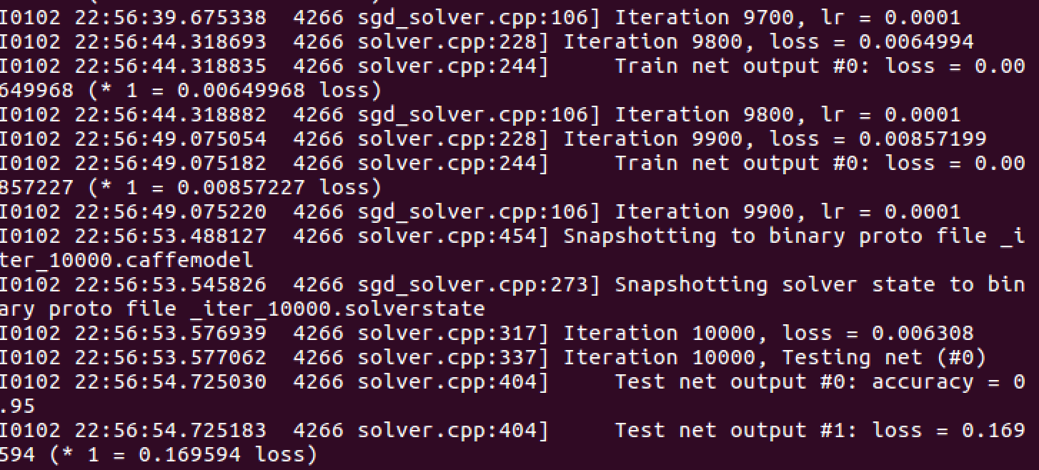
心得体会
caffe本身是简单易用的,但是若对神经网络本身算法原理一窍不通,就无法设置合适的参数,来提高图片识别的准确度。因此,在熟练使用工具的基础上,还要加强对算法原理的了解掌握,这两者是相辅相成的关系。